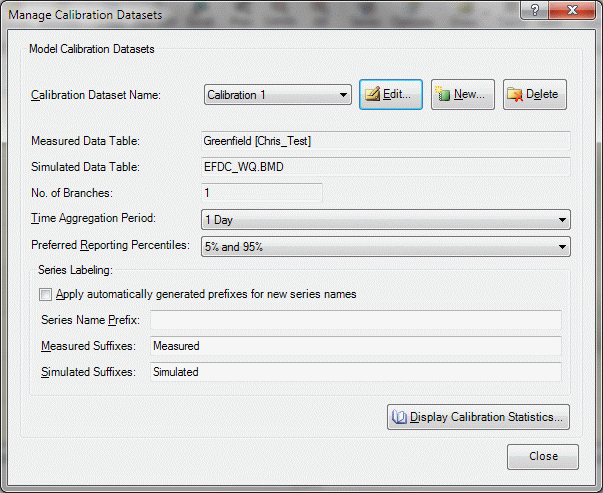
Calibration datasets are paired data tables of any type that are displayed simultaneously. They are useful to compare modeled to observed results, perform data aggregation in time and space, calculate statistics, and prepare report-ready multi-graph figures. Calibration datasets are a powerful but complex feature of Graph normally used only by water quality modelers for post-processing.
First, you must open the data files or tables that contain the measured and simulated results. You then define a Calibration dataset by giving it a name and assigning the measured and simulated data tables. Do this using File | Data Files & Tables | Manage Calibration Datasets and then click the New button; the calibration dataset name will default to "Calibration n" where n is one plus the number of existing calibration datasets. These can be renamed to suit your needs. Note: you can also access this feature from the Manage Data Series form by clicking the Build button and selecting Manage Calibration Datasets.

As discussed in Getting Help, click on the question mark and then one of the form controls (or move to the control using the TAB key and press F1) to get context-sensitive help for this very busy form.
When you add or edit a calibration dataset, the Model Calibration Table Mapping form will appear which allows you to define pseudo stations and parameters to stations and parameters in existing tables containing measured and simulated results; these are known as Aggregated Data Stations and Parameters because you may wish to assign multiple measured stations or simulated grid cells to the same pseudo station (for example, if multiple sampling locations are located within the same grid cell or if a comparison of grid multiple cells will be made to a given sampling station). When multiple stations or cells are selected, the average values for all data is computed and plotted.
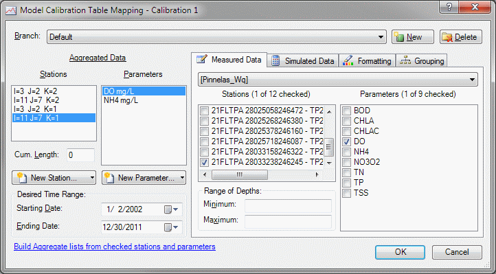
This form employs an extra amount of heuristics to make it easier to assemble your list of desired aggregated data pseudo stations and parameters. Here is a sample procedure:
Select the previously opened data table from the drop-down list (e.g., Chris_Test) if it wasn't automatically selected for you; the list of available stations and parameters will automatically be filled with the available values. Note that you may have have multiple tables open, so make sure to select the appropriate table.
Check all stations and parameters in the Measured Data table that you want to add to the Aggregated Data list, then click the Build Aggregate lists from checked stations and parameters line (or click the down arrow next to the New Station button and select New from Checked); all combinations will be added to the lists (which can be later edited).
If you want to filter the WRDB measured data so that only data within a specified range of depths are included, indicate that range in the Range of Depths box; leave blank to include all data regardless of depth (or if depth information is not available).
After all Aggregated stations and parameters have been created and mapped to measured data, do the same with simulated data; this tab will look different depending on the type of table selected (it will usually be BMD). Initially the tab will look like this:
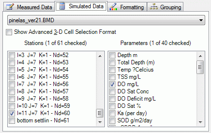
If a specially formatted BMD file created from a 3-D model like WASP or EFDC is detected the Show Advanced 3-D Cell Selection Format checkbox is visible; when checked an advanced format for selecting ranged of I, J, K cells is available:
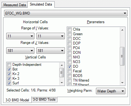
Select the range or i, j, and k indices which define the box which will be associated with the selected Aggregated Data station as well as the BMD parameter to be associated with the selected Aggregated Data parameter. You may also want to select which BMD parameter to use to weight the values that are averaged. This is useful if you want to volume average a parameter, such as DO, over a range of cells.
The Assign to All Stations item under the New Parameter button allows you to quickly assign parameters once you cross connect the initial parameter. A quick way to accomplish the assignments if you have multiple stations is to first assign i,j,k grid cells to all the stations. Then select one station and assign each parameter to the appropriate simulated parameter, after each assignment select the assign to all station function (under the New Parameter button) and this parameter assignment will be the automatically assigned for all the stations.
There is another shortcut to building multiple aggregate stations and parameters: with the list of Aggregate Stations empty, on either the Measured or Simulated Data tab check all the desired measured or simulated stations and parameters and then click the "Build Aggregate lists..." link at the bottom of the form. This will add combinations of stations and parameters to the aggregate lists and assign the checked measured or simulated stations and parameters. All that must be done then is to manually map the unassigned stations and parameters. For example, if you use a set of measured stations and parameters to build the aggregate lists, you will have to manually assign the simulated stations and parameters.
Although calibration datasets will normally be used to plot time series comparisons and compute overall statistics, you can also plot profiles by creating pseudo branches of measured stations and simulated grid cells. For example, if you want to create a plot of computed and observed values at the surface along the centerline of a 3-D estuary, do the following:
Click the New button and enter the name of the desired "branch"
As previously described, selected the measured data stations that are located along the centerline and the parameters of interest; click Build Aggregate lists...
If desired, enter the depth range for each stations (e.g., 0 to 5 meters)
For each Aggregate Station, enter a value for the Cumulative Length (so that profile plots can be made)
On the Simulated Data tab, click the 3-D BMD Tools tab; paste in the information regarding cell sizes (from the EFDC data file), specify the type ofr branches to build, the J (or I) indices associated with each longitudinal or transverse profile, and a comma-separated list of desired parameters:
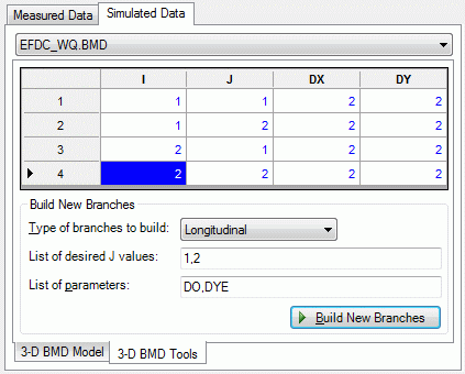
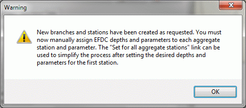
After clicking Build New Branches, the following message appears:
Graph allows you to predefine formatting characteristics to series that will be created from calibration datasets. This helps you to create consistent looking graphs from calibration data. The Formatting tab looks like this:
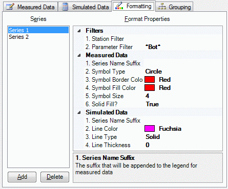
Normally, you will define formats for only a single series (that series created by any of the Aggregate Station/Parameter pairs. Using the form, configure the formatting for the lines associated with simulated data and symbols associated with measured data. These formats will be used whenever a new series is added using any of the Aggregate station/parameters from this calibration dataset (instead of the default series formats).
If you wish to automatically use different formatting depending on the aggregate station name, you can define multiple series formats and specify Station and Parameter Filters. For example, suppose you want to plot surface and bottom measured and simulated data using different colors and/or symbols (perhaps so they can both be added to the same graph using Tools | Build Graphs). As shown above, the WASP station names always end with "K=2" for surface cells and "K=1" for bottom cells. Therefore, enter "*K=2" for the Station Name filter (* is the wildcard character) and "Surface" for the Series Name Suffix. Series 2 would have similar entries to identify the bottom stations. Add as many formatting series as unique station names.
BMD files created using EFDC encode data at various depths (K values) using Parameter names. These can be accomodated by using the Parameter Filter. For example, enter "*Bot*" to use only those parameters containing the string "Bot".
Note: if the Station or Parameter Filter is blank, the formatting for that series will be used if no other series Filter matches the station/parameter name.
If you intend to automatically plot multiple series when building graphs, each with their own format, you must also properly configure the Grouping tab:
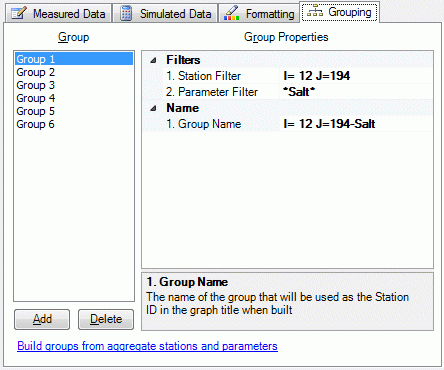
If you wish to automatically plot multiple series on the same graph tab when building graphs (each with their own format), you can define multiple series formats using Station and Parameter Filters, then configure how the multiple series will be chosen using the Grouping tab. For example, suppose you want to automatically add both surface and bottom measured and simulated data to the same graph (using Tools | Build Graphs). As shown above, the series formats have been defined. Next, define how to group multiple Aggregate stations and parameters on a graph by indicating the station and parameter filters for groups. This is accomplished by entering names with wildcard characters.
As with the Formatting tab, BMD files created using WASP will only require a Station Filter, but BMD files created using EFDC will require both a Station and Parameter filter to work correctly.
It can be tedious to manually create groups for BMD files having many stations and parameters. Click the Build groups from aggregate stations and parameters link to have WRDB Graph do this for you. Because the Group Names are formed using the Aggregate Parameter and Station names, and graph titles may be taken from the Group Names, you may want to rename the Station and Parameter names (by right-clicking on a selected item) before using the Build groups... link.
After calibration datasets are created, they can be selected from the list of open tables in the Manage Data Series form and will have names like "Calibration: Calibration 1". When selected, the list of Aggregate (pseudo) stations and parameters that you created will appear. Because all the mapping of stations (or cells) and parameters has already been done, adding a data series will plot measured data as symbols and simulated data as lines according to the formatting previously defined. Note that you can override these settings on the Properties Panel, Series tab (see Using the Graph Control).
The data that will actually be plotted are averages (or weighted averaged) of data from all stations or cells assigned to each Aggregate stations. Furthermore, if the Time Aggregation Period on the Manage Calibration Datasets form is not None, then time aggregation will be done.
Calibration statistics are automatically computed for each Aggregate Station and Parameter; these statistics can be displayed on the graph or a Calibration Report can be prepared. To see available calibration reports, click the Display Calibration Statistics button on the Manage Calibration Datasets form; the following will appear:
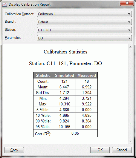
These are HTML reports that can be copied to the clipboard and pasted into a report or spreadsheet; these reports are also available when creating named print layouts (and can automatically be created when building graph tabs using calibration datasets).
As suggested by the controls on the form, you can create individual calibration reports for any existing calibration dataset, branch, Aggregate Station, and Aggregate Parameter by selecting from drop-down lists, and a report will appear which looks like the one above. An additional option on the Station list is All Stations--Long Report) which gives a consolidated report for all stations that looks like this:
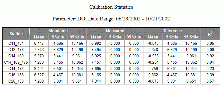
Note that only this report utilizes the Preferred Reporting Percentiles selection on the Manage Calibration Datasets form.