Calculation
Graph Type
Description
Constant Value
Time Series,
Longitudinal, Depth & Width Profiles
Based on constant value that you specify
PCode Criteria Limit
Time Series,
Longitudinal, Depth & Width Profiles
For WRDB tables, extracts the Criteria Limit value for the selected series' PCode and plots the constant value.
Moving Average
Time Series
After prompting for the number of periods in the moving average, computes the series; data points are plotted at the center point of the number of periods. Available periods are:
|
Number of Adjacent Points Averaged |
Purpose |
|
24 |
Hourly Data to Daily Average |
|
168 |
Hourly Data to Weekly Average |
|
7 |
Daily Data to Weekly Average |
|
30 |
Daily Data to Monthly Average |
|
3 |
Monthly Data to Quarter-year Average |
|
6 |
Monthly Data to Half-year Average |
|
12 |
Monthly Data to Annual Average |
Please note that the moving average plot is based upon the number of consecutive numbers averaged. A true daily average will be computed from hourly data only if there are no missing data points and the data start at 12:00 a.m. Nevertheless, the moving average plots can be very helpful for screening out the "noise" in the data and help you see underlying trends and relationships.
Daily Averages
Time Series
Calculates average daily values for all data found within each day and plots them at noon.
Sine Curve Fit
Time Series
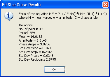
Uses a non-linear curve fitting tool to fit a sine curve to the observed data. This is most useful when applied to daily, weekly, or monthly average data to discern annual periodicities. When you click this button, a non-linear fit routine is started which determines the sine curve coefficients which best fit the data:

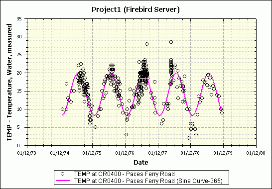
This is the same equation used by Dyar and Alhadeff in Stream-Temperature Characteristics in Georgia, USGS WRI Report 96-4203. The resulting sine curve are thereafter displayed like this:

Adjust by Constant Value
Time Series,
Longitudinal, Depth & Width Profiles
Creates a new series by performing an arithmetic calculation on the selected series; you can specify the operator (+,-,*,/) and a constant to be used.
Add Two Series
Time Series,
Longitudinal, Depth & Width Profiles
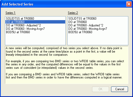
Presents the Add Selected Series form in which you can select the two series to be added:

Subtract Two Series
Time Series,
Longitudinal, Depth & Width Profiles
See Add Two Series, above.
Linear Fit
Scatter Plot
Fit least-squares linear fit to data in the form y=Ax + B
Power Fit
Scatter Plot
Fit least-squares linear fit to data in the form y=Ax^B
Exponential Fit
Scatter Plot
Fit least-squares linear fit to data in the form y=A Ln(x) + B
Normal Distribution
Probability
Fit normal distribution to observed data.
Log-normal Distribution
Probability
Fit log-normal distribution to observed data.
Log-Pearson III Distribution
Probability
Fit Log-Pearson III distribution to observed data.